A Guide to Utilizing PivotTables in Excel for More Intelligent Data Analysis

As someone who works with huge data sets in Excel, you are aware of how intimidating it may be to have an unending number of rows and columns. In Excel, the PivotTable function enables you to rapidly summarize, analyze, and show data in a manner that is both obvious and useful. This is accomplished without the need to manually filter and calculate the data. For more intelligent decision-making, it is one of the most powerful tools that Excel has to offer.

This is a PivotTable, right?

An example of a dynamic table is a pivot table, which allows you to reorganize and summarize data without affecting the dataset that was first created. Grouping, filtering, and calculating numbers may be accomplished with only a few clicks, which makes it simple to identify patterns and insights.

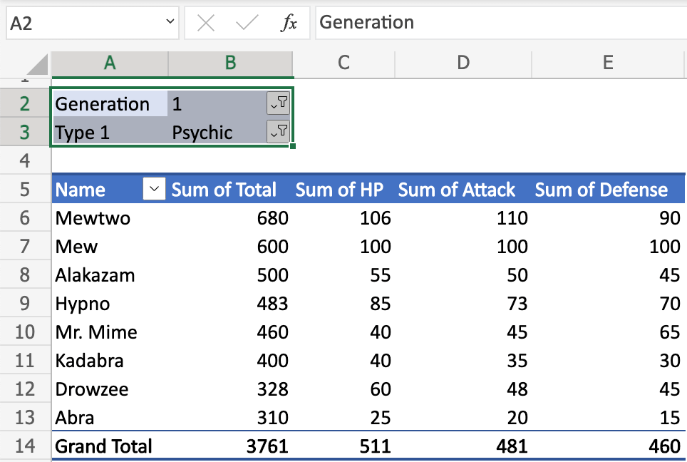
A PivotTable, for instance, may rapidly display you the following information, rather than requiring you to read through thousands of sales transactions:

The sum of sales for each area.
Product category sales broken down.
Charting the patterns of monthly or quarterly revenue.

Are PivotTables Worth Using?

PivotTables are better at improving accuracy and saving time by:

The ability to swiftly summarize data by dragging and dropping fields.
Patterns that you may overlook while working with raw data are highlighted.
Calculating things like sums, averages, or percentages with the use of automation.
Developing interactive reports that become current when the data undergoes changes.

1. Insert a PivotTable.

Make sure that your dataset has headers before selecting it.

Locate the Insert → PivotTable tool.
Make your selection for the location of the PivotTable (a new worksheet is recommended).
When you look to the right, you will find a PivotTable that is empty and a field list.

2. Understanding PivotTable Areas.

To use a pivot table, just drag and drop certain fields into the appropriate sections:

Categories that you want to group by, such as Region or Product, are represented by rows.
Columns are subcategories that need to be compared, such as the year and the month.
Valuations are numbers that may be summarized, such as the total sales or the average quantity.
Filters are criteria that are used to filter down the results, such as displaying just 2024 data.

3. Construct a Basic Report

Taking a look at the historical sales data

Move the Region to the Rows.
Position the Product Category in the Columns.
Move the Sales Amount to the Values tab.
At this point, you have a table that is able to compare sales quantities according to product category and location.

4. Apply Slicers and Filters to the Data

PivotTables become more interactive when filters are in use:

You may narrow down your search to certain years, goods, or personnel by using the Filter box.
To create clickable buttons that immediately filter your data, you may add Slicers by using the Insert → Slicer command.

5. Utilize PivotCharts to Gain Visual Insights

A PivotChart is a visual representation of a PivotTable that is simple to read.

Use your PivotTable to choose it.

Navigate to the Insert → PivotChart menu option.
Pick a kind of chart (column, bar, line, or pie) to use.
It is now possible to filter the PivotTable, which will result in the chart automatically updating.

6. Values should be summarized in a variety of different ways.

Although PivotTables employ SUM by default, you have the ability to modify this:

Take a right-click on a value field and choose Summarize Values By.
Options include Count, Average, Maximum, Minimum, and Percentage of Total, among others.
This opens the door to further in-depth analysis without the need to write formulae.

7. Refresh with New Data.

Right-click the PivotTable and pick the Refresh option if the data that you are using as a source changes.

You may want to think about utilizing a Table as your data source for ongoing reporting so that the PivotTable can extend and contract automatically.

8. The Most Effective Methods for PivotTables

Always check to ensure that the headers of your source data are clear.
Maintain the data in a tabular structure (no cells should be combined).
To improve readability, rename the fields and the results.
Play around with dragging fields; you won’t need to worry about breaking anything.

When it comes to dealing with Excel, pivot tables are a game-changer at every level. Analysis and summarization of data may be performed in a matter of seconds, as opposed to manually crunching statistics. Your reports will not only be more intelligent, but they will also be simpler to comprehend if you make use of characteristics like as filters, slicers, and PivotCharts. After becoming proficient with pivot tables, you will wonder how you ever managed to function without them.

Tags: A Guide to Utilizing PivotTables in Excel for More Intelligent Data Analysis